Fluid Solver

This one has been a long time coming. Inspired by this 10 minute physics video and molded by about a year or so of confusion. I wanted a fluid solver, no… the geometry nodes fluid solver!

And now I have it:

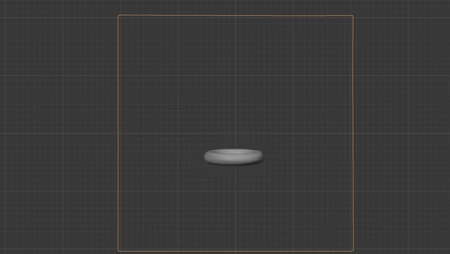
Unlike the typical approach to making a fluid solver, mine does not use a staggered grid. I don’t like it. I won’t be a part of the problem. I stand on the right side of history. Instead:

I’ll be simulating on a collocated grid

That’s fancy-speak for a grid where the info is stored at the center of the grid voxels. Not the faces. Much more natural in my not-so-humble opinion.

Please lubricate your brain for some vector math. Let’s start easy. The simulation loop for every frame is just:

Advect both the density and velocity (along the velocity grid)

Add forces to velocity

Remove divergence from the velocity grid (this is called ‘projection’)

Repeat

The crux of this method, the interesting part, is step 3. What you have to know is that:

Fluids are incompressible

Meaning, fluid is neither created nor destroyed. A conservation of mass. It can’t come from nowhere, or, compress into nothing. This can be enforced by ensuring:

\[\nabla\cdot\vec{V} = 0\]

That is, no divergence. Fluid should just curl, not expand or contract. We need some way to remove all divergence from $\vec{V}$ on every iteration. Enter Helmhotz Decomposition (a nice residue from the much too confusing Hodge Decomposition). Helmhotz deals us the good stuff. The key to the puzzle. He says word on the street is that any $\vec{V}$ can be decomposed (for our purposes) into:

\[\vec{V} = \st{curl}_{V} + \st{div}_{V}\]

Meaning a curl free part and a divergence free part. And now, the second key insight. For any curl-free field:

\[\st{curl}_{V} = \nabla(\phi) \quad \text{for some scalar } \phi\]

Weird… but useful! Let’s bring that in:

\[\vec{V} = \nabla(\phi) + \st{div}_{V}\]

And mysteriously take the divergence of both sides:

\[\nabla\cdot\vec{V} = \nabla\cdot\nabla(\phi) + \nabla\cdot\st{div}_{V}\]

And what do you think the divergence of a divergence free field is ☺️

\[\nabla\cdot\vec{V} = \nabla\cdot\nabla(\phi)\]

This bad boy is called the Poisson Equation, and it’s solvable! We’re going to calculate some fancy iterations to find $\phi$, and then, recover the divergence free part.

Now, you can do the derivation yourself. As punishment. Out of a masochistic urge. But, I actually did it for you, on the back of a paper plate in an Orlando resort (my wife and I demolished Universal Studios).

But trust me, if you take the derivates in the right way (with a tiny time-step $h$) and you’ll end up with:

\[\phi_{x,y,z} = \frac{\sum\left(\phi_\text{neighbors}\right) - \nabla\cdot\vec{V}}{6}\]

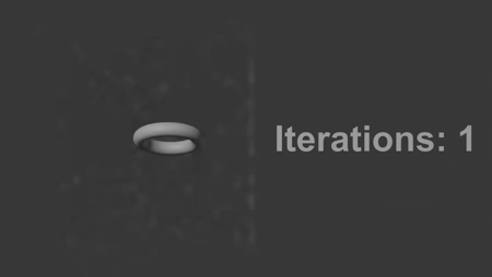
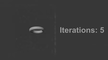
In 3D, $\phi$ will have 6 voxel neighbors (up, down, left, right, forward, back). Just initalize $\phi=0$ to start, and plug it in over and over again (in parallel). Like 20-100 times per frame. This by the way is called a Jacobi solver.

Phew. Finish off with:

\[\st{div}_{V} = \vec{V} - \nabla(\phi)\]

Bad-a-bing, bad-a-boom, you removed your divergence. At least most of it. There are some fine details, but that is why I made a tutorial 😉

Also, make sure to pick up the project file (above) for a much more refined version!